
2023-07-02, Johannes Köppern
When I started my work in predicting crop yields for a field, I found myself delving into the various factors that influence these yields. I soon realized that variables like temperature, rainfall, and soil quality play crucial roles in determining crop yields, and that these variables can interact with each other in complex ways, including higher powers and combinations. Naturally, I wanted to find a way to extend the simplicity and transparency of a 1D polynomial fitting function like np.polyfit to handle higher-dimensional polynomials.
So, I embarked on a journey to develop an approach that could handle these multidimensional relationships while maintaining the simplicity and transparency of np.polyfit. With the help of explanations from other posts and my own insights, I came up with a method that achieves this goal. In this article, I’ll share my hands-on approach to fitting higher-dimensional polynomials to predict crop yields, taking you step by step through the process I developed. Let’s dive in (after a short excursion how to fit 1D polynomials in data with Numpy) and explore the world of multivariate polynomial regression together!
Fitting 1D polynomials with Numpy
For fitting polynomials that depend on only one variable (let’s call this x) there is a simple usable function with numpy.polyfit. For example, the polynomial could model the correlation between the measured variable y and the independent variable x by \(y = c_0 + c_1x +c_2x^2\).
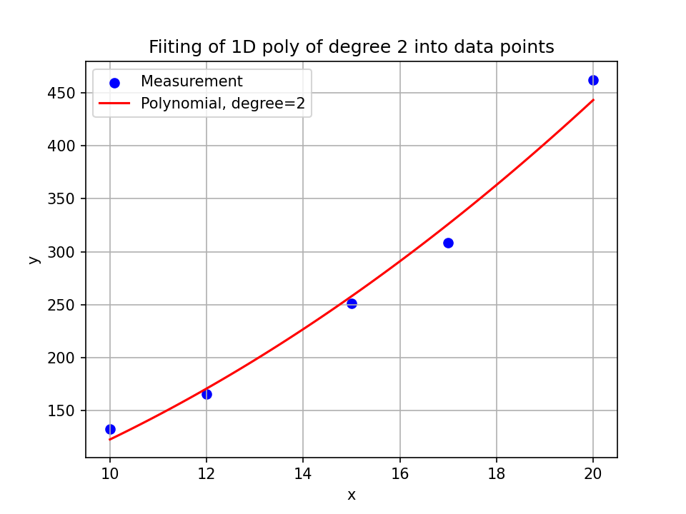
For example, we might have measured air pressures \(\mathbf{y}=[132.98972399, 165.76948266, 251.1865844 , 308.51061146,462.16877899]\) at temperatures \(x=[10, 12, 15, 17, 20]\) five times (this example is constructed). With
p_est = np.poly1d(np.polyfit(x, y, deg=2))
we determine \(p_{ \rm{est}} \) to be
and we model out data with this polynomial. With it, we can map any \(x\) to a \(y_{\rm{est}}\) and we thus model the relationship between the two quantities.
You can find the python file I wrote to create this plot here.
Formulation as set of linear equations (1 independent variable)
Our task in polynomial fitting (whether we consider a one-dimensional polynomial or one with several independent variables) is to choose the coefficients \(c_i\) that the polynomial lies as well as possible in the data. Here we define this good in the sense that any distance (error) between our polynomial \(p_{\rm{est}}(x_i)\)’s value and the corresponding data point’s value \(y_i\) becomes as small as possible. To do this, we square each error and sum these squares to form the criterion \(c\):
Since \(p_{\rm{est}}\) of the coefficients \(c_i\), we can minimize the criterion \(c\) by their choice and we find thereby the optimal choice of those coefficients according to the criterion \(c\).
The optimal choice of coefficients is called solving an optimization problem. And for this task mathematical algorithms exist, which are available in libraries, like Numpy, to the programmer.
Note: It is always important (not only in mathematical optimization tasks) to define the terms good, better and worse precisely. Otherwise, the task cannot be processed and a statement such as one car is better than the other is meaningless. The question can or should always follow: With regard to which criterion?.
So, let’s write our optimization problem in a form suited for mentioned optimization algorithms:
We can formulate our problem as a linear system of equations of the form
(although the polynomial itself is non-linear). Here \(\textbf{c}\) is the vector of the searched coefficients, \(\textbf{y}\) are the one component of the measuring points (\(y_i\)) and into the matrix \(\textbf{A}\) goes in each case the Other component of the measuring points,
To solve optimization problems \(\textbf{Ac}=\textbf{y}\) for example the function `numply.linalg.lstsq` exists (lstsq stands for least-squares, as our criterion is defined as the sum of squared errors and this should be minimized). But first let’s see how the matrix \(\textbf{A}\) is constructed and how we determine it to pass it to the optimization algorithm.
Each measurement (each pair of \(x_i\) and \(y_i\)) contributes an equation to the optimization problem. For simplicity, consider our first example, that is, a second degree polynomial in only one variable (\(x\)), which produces \(y_i= 1 + 2x_i + 3x_i^2\). Thus the vector of coefficients is
thus a column vector. According to the equation \(\mathbf{Ac}=\mathbf{y}\), the element \(y_i\) results from multiplying the \(i\)-th row of \(\mathbf{A}\) by the vector \(\mathbf{c}\):
We can calculate the necessary pots of our measured variables \(x_i\) (after the measurement and before setting up the optimization problem) and build the matrix \(\mathbf{A}_{\rm{example}}\) with them:
\begin{bmatrix}
1 & x_0 & x_0^2 \\
& .. & \\
1 & x_i & x_i^2 \\
& … & \\
1 & x_n & x_n^2
\end{bmatrix}
\)
if we conducted \(n\) measurements.
Thus, for \(y_i\) we get \(y_i=c_0 + c_1x_i+c_2x_i^2\), which is exactly our polynomial (our model).
OK, for a problem with one independent variable \(x_0\) we build the (linear) optimization problem for a nonlinear polynomial. Now, in the next section, we can take on a polynomial with multiple independent variables \(x_0,x_1,x_2,…\).
Formulation as set of linear equations (multiple independent variables)
In the following we will take two examples of the formulation of a polynomial with two independent variables. The next section then implements these polynomials with Python.
(Example 1) Let’s start again with an example: Suppose there are two independent variables \(x_0\) and \(x_1\). Furthermore, we define that our polynomial \(p_1\) has degree 2 and that each power of \(x_0\) is to be multiplied by each power of \(x_1\):
\tag{eq:p1}\)
Before setting up the optimization problem, we can calculate the dependent variables, such as \(x_0x_1\) or \(x_0^2\). These are new features, so we are doing feature engineering. Which features are relevant (i.e., which should be included in our polynomial) depends on the problem at hand. And with them we can set up the matrix \(\mathbf{A}_1\) of our optimization problem, which is multiplied by \(\mathbf{c} := [c_0,c_1,..,c_8]^{\rm{T}}\):
\begin{bmatrix}
1 & x_{0,0} & x_{0,0}^2 & x_{0,0}x_{0,1} & x_{0,0}x_{0,1}^2 & x_{0,0}^2x_{0,1} & x_{0,0}^2x_{0,1}^2 & x_{0,1} & x_{0,1}^2 \\
1 & x_{1,0} & x_{1,0}^2 & x_{1,0}x_{1,1} & x_{1,0}x_{1,1}^2 & x_{1,0}^2x_{1,1} & x_{1,0}^2x_{1,1}^2 & x_{1,1} & x_{1,1}^2 \\
&&&& \dots \\
1 & x_{n-1,0} & x_{n-1,0}^2 & x_{n-1,0}x_{n-1,1} & x_{n-1,0}x_{n-1,1}^2 & x_{n-1,0}^2x_{n-1,1} & x_{n-1,0}^2x_{n-1,1}^2 & x_{n-1,1} & x_{n-1,1}^2
\end{bmatrix}
\)
The number of rows of \(\mathbf{A}_1\) (\(n\)) is equal to the number of measurements, that is, how many triples \((x_{0,i},x_{1,i},y_{1,_i})\) are present in the data.
The vector \(\mathbf{y}_1 := [y_0,y_1,…,y_{n-1}]^{\rm{T}}\) is composed of the measured quantities \(y_{1,i}\) and it can thus be set up without further ado.
Then the optimization task is completely formulated and the formulated optimization problem can be solved for \(\mathbf{c}_1\).
How this solution can be done in Python is shown in the next section.
For other polynomials, i.e. with a different number of independent variables and a different structure (i.e. which quantities are multiplied to which powers), a matrix \(\mathbf{A}\) can be set up analogously.
(Example 2) An example of another polynomial, which will also be implemented with Python in the next section, is.
\)
This leads to
\begin{equation}
\mathbf{A}_2(x_0,x_1): =
\begin{bmatrix}
1 & x_{0,0} & x_{0,0}^2 & x_{0,0}x_{0,1} & x_{0,1} & x_{0,1}^2 \\
&&&\dots
\end{bmatrix}
\end{equation}
\)
The polynomials \(p_1\) and \(p_2\) differed because we each took different paths during the feature engineering step.
In the next section, we can now implement the systems of equations according to these definitions in Python and thus set up \(\mathbf{A}_i\) and \(\mathbf{y}_i\), respectively. Afterwards, we can use Python to solve the systems of equations and calculate the coefficients \(\mathbf{c}_i\).
Fitting with Python

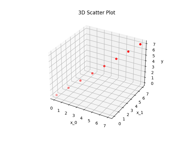
Both polynomials \(p_1\) and \(p_2\) are fitted into the points
x = [(0,0),(1,1),(2,2),(3,3),(4,4),(5,5),(6,6),(7,7)]


y = np.array([0,1,2,3,4,5,6,7])
as depicted in the following figure:
This is done by the following Python code:
import numpy as np
import matplotlib.pyplot as plt
from mpl_toolkits.mplot3d import Axes3D


x = [(0,0),(1,1),(2,2),(3,3),(4,4),(5,5),(6,6),(7,7)]
y = np.array([0,1,2,3,4,5,6,7])
degree = 3


degrees_1 = [(i, j) for i in range(degree + 1) for j in range(degree + 1)]
degrees_2 = [(i, j) for i in range(degree + 1) for j in range(degree + 1 - i)]


print("degrees_1", degrees_1)
print("degrees_2", degrees_2)


A_1 = np.stack([np.prod(np.array(x)**np.array(d), axis=1) for d in degrees_1], axis=-1)
A_2 = np.stack([np.prod(np.array(x)**np.array(d), axis=1) for d in degrees_2], axis=-1)


print("A_1", A_1)
print("A_2", A_2)


c_1 = np.linalg.lstsq(A_1, y)[0]
c_2 = np.linalg.lstsq(A_2, y)[0]


print("c_1", c_1)
print("c_2", c_2)
The scipt’s output is:
degrees_1 [(0, 0), (0, 1), (0, 2), (0, 3), (1, 0), (1, 1), (1, 2), (1, 3), (2, 0), (2, 1), (2, 2), (2, 3), (3, 0), (3, 1), (3, 2), (3, 3)] degrees_2 [(0, 0), (0, 1), (0, 2), (0, 3), (1, 0), (1, 1), (1, 2), (2, 0), (2, 1), (3, 0)] A_1 [[ 1 0 0 0 0 0 0 0 0 0 0 0 0 0 0 0] [ 1 1 1 1 1 1 1 1 1 1 1 1 1 1 1 1] [ 1 2 4 8 2 4 8 16 4 8 16 32 8 16 32 64] [ 1 3 9 27 3 9 27 81 9 27 81 243 27 81 243 729] [ 1 4 16 64 4 16 64 256 16 64 256 1024 64 256 1024 4096] [ 1 5 25 125 5 25 125 625 25 125 625 3125 125 625 3125 15625] [ 1 6 36 216 6 36 216 1296 36 216 1296 7776 216 1296 7776 46656] [ 1 7 49 343 7 49 343 2401 49 343 2401 16807 343 2401 16807 117649]] A_2 [[ 1 0 0 0 0 0 0 0 0 0] [ 1 1 1 1 1 1 1 1 1 1] [ 1 2 4 8 2 4 8 4 8 8] [ 1 3 9 27 3 9 27 9 27 27] [ 1 4 16 64 4 16 64 16 64 64] [ 1 5 25 125 5 25 125 25 125 125] [ 1 6 36 216 6 36 216 36 216 216]


5.00000000e-01 -1.37390099e-15 -1.11022302e-16 -1.37390099e-15 -1.11022302e-16 -1.11022302e-16]


Quadratic Fitting Error (c_1): 2.886173008969347e-22
Quadratic Fitting Error (c_2): 1.3075027753669353e-25
And this is how \(p_{1/2}\) lie in the \(x_0-x_1-y\) plane:
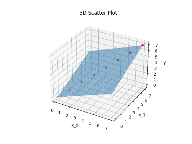
Let’s talk about the quadratic fitting errors
| Polynomial | Error |
|---|---|
| \(p_1\) | 2.886173008969347e-22 |
| \(p_2\) | 1.3075027753669353e-25 |
Both errors are zero except for numerical residuals. That means that both polynomials run exactly through the given points. This is possible because they both have more parameters \(c_{1/2,i}\) than points given for the regression.
Conclusion
With the polynomial that way identified, I was thus able to model the relationship between moisture in a field, temperature and crop yield. And this was done by means of a model which, on the one hand, is easy to evaluate numerically and, on the other, is comprehensible.
Alternatively, I could have identified a neural network as a model, for example. It would have represented the connection just as well, but in the result would not have been more traceable. The neuronal net would be a opaque block into which named humidity and named temperature enters and the yield comes magically out. How it comes to its result would not have been understandable, however, differently than with my polynomial. (Note: That a neural network can approximate a polynomial function is stated by the universal approximation theorem. So if a polynomial describes a relation completely, a neural network can describe the same relation, but it offers no added value, the relation would already be described completely by the polynomial).
The method shown here leaves every freedom concerning the structure of the polynomial to be identified. And so I use the source code shown above whenever I want to identify a polynomial as a model.
Many thanks to DALL·E 2/Bing for pictures!